The attractor curve is one of those captivating effects we can create in Grasshopper that brings our designs to life. The attractor curve algorithm allows us to manipulate and control a series of objects in response to a curve, adding a new dimension of interactivity and creativity to our work.
In this article we are going to learn the logic behind attractor scripts, learn how to set up an attractor curve in a script step-by-step.
Let’s get started!
The Logic Behind the Attractor Curve
Before we dive into which Grasshopper components to use, it’s important to understand the logic behind the attractor curve effect.
Let’s start by defining what we mean by “attractor curve”.
In an attractor curve script, a series of objects, which we’ll refer to as a “field,” ‘react’ to a curve (or other object), by modulating the extent of a geometric transformation. The outcome is a visual effect of a gradient or smooth transition.
Now what’s behind this effect?
In essence, the attractor curve effect in Grasshopper works by remapping objects’ distance to a curve, to a geometric transformation we define. This could be something as simple as scaling or rotation, or a more complex series of geometric operations.
Creating a curve attractor effect can be done in four steps:
- Create a field of objects
- Set up a geometric transformation for the objects in the field (for example a rotation)
- Calculate the distance from each object to the attractor curve
- Remap the resulting distances to transformation values
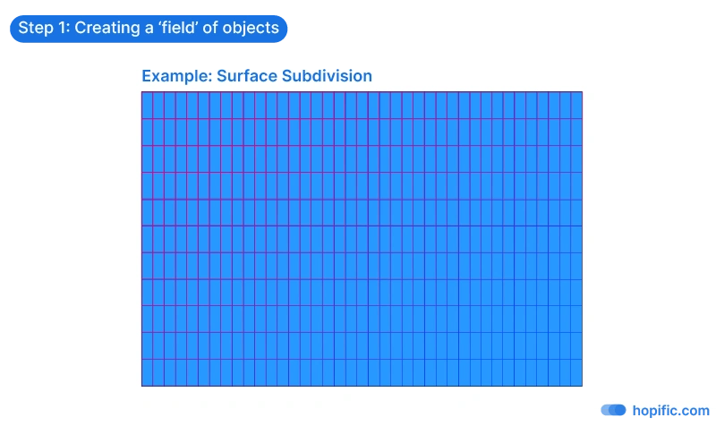
Step 1. Create a field of objects
For the attractor curve effect in Grasshopper to be recognizable, we need a certain number elements to apply this effect to. We need to create a field. It can be a linear array or a two-dimensional grid of elements, which is what we’ll use in this example.
Since gradient effects already create visual complexity, the fields we apply them to are usually quite simple and regular.
Step 2. Define a geometric transformation for the objects in the field
Once we’ve set up our field, the next step is to define the transformation.
What is the geometric transformation that the gradient is going to control?
The attractor script will transform each element in the field by it’s own dedicated value.
The transformation can be as simple as the scaling or rotation of an object. But it can get much more complex, it could be a series of geometric operations – the important thing is that at the end the whole transformation can be controlled by a single number. This is essential for the next step.
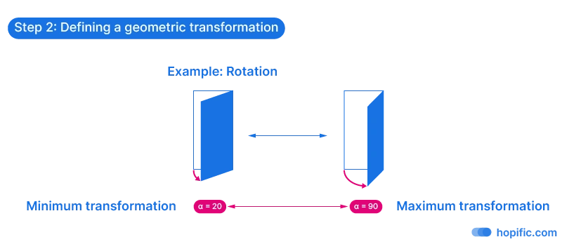
As we define the transformation, we will also need to define a minimum and a maximum state for this transformation, in the example we’ll use, it will be a minimum and maximum rotation value.
The objects in the field closest to the attractor curve will get the minimum transformation, and the ones farthest from the curve the maximum transformation (or vice-versa).
Step 3. Define a distance that will drive the transformation
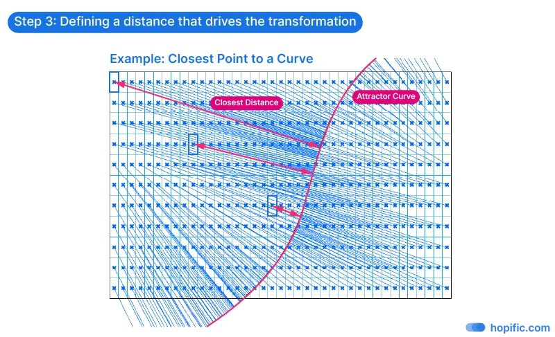
The third and crucial step to create an attractor curve effect in Grasshopper, is to define a distance relationship between the objects in our field and the attractor geometry. These distance values will act as the transformation driver.
The distance from each element in the field to the attractor curve will drive the extent of the transformation. Since the distance will be different for each object, each transformation value will be unique, resulting in a gradual, nuanced transformation effect.
To calculate the distance from an attractor curve to each object in the field, we need a point that represents each object. This point will act as a proxy for the distance calculation. The point can be generated in a number of ways, for instance by getting the centerpoint of each object.
It doesn’t matter whether the reference point is on top, the center, or the bottom of the elements, as long as the point is generated the same way for all elements in the field.
The resulting distance values are going to have a minimum and maximum value, the minimum value representing the elements closest to the attractor curve and the maximum value the most distant ones.
Step 4. Remap the distance to the transformation
The final step that brings the gradient to life, is to create a relationship between the distance values and the extent of the transformation (for example a rotation).
Both the distance values and the transformation values are numbers, each with their own minimum and maximum ranges.
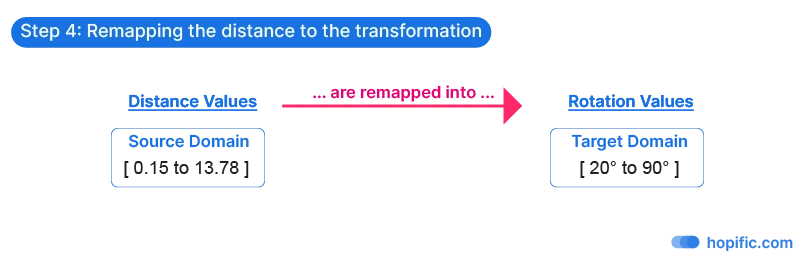
By remapping the distances from the distance range to the transformation range, we create a proportional relationship between the two.
Remapping a number means that we take a number that exists within one numerical domain and remap it to another numerical domain, proportionally.
Finally, we can use the resulting, remapped values to drive the object transformation (rotation) we set up in step 2 to finalize our attractor curve gradient!
Let’s learn how this attractor curve logic can be broken down into components inside Grasshopper!
Attractor Curve Step-by-Step Tutorial
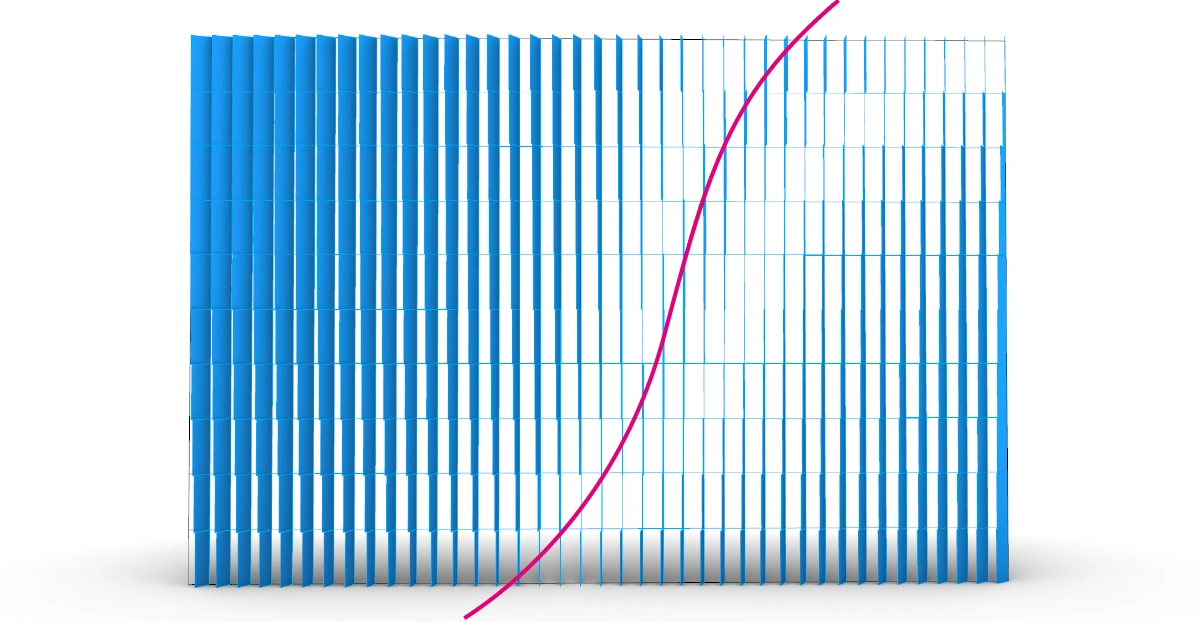
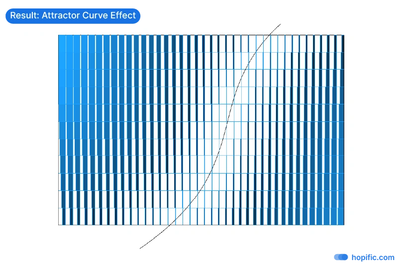
As an application example for an attractor curve in Grasshopper, we’ll be creating the example introduced above: a simple façade consisting of vertical panels rotated in relation to the distance to a curve.
Subdividing a surface to create an object field
Let’s start by creating a simple rectangular grid. We’ll do so by subdividing a surface.
We’ll draw a vertical rectangle that’s 60 units wide and 40 units tall, and reference it to a Curve container in Grasshopper.
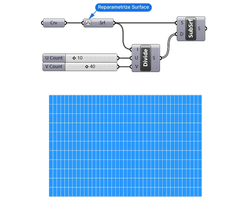
Let’s add a Surface container to create a surface from the curve, and let’s reparameterize the surface to make sure we start with a clean slate. To do that, right-click on the left-hand input of the Surface container component, and toggle ‘Reparameterize’.
To subdivide the surface – let’s add both an Isotrim (SubSrf) and a Divide Domain² component.
Then let’s plug the surface into both S input of the Isotrim as well as the I input of the Divide Domain² component.
By default the surface domain has 10 subdivision in both the U and V direction. Let’s add two number sliders to adjust that. Let’s go with 10 for the U and 40 for the V input.
Depending on how we created the curve, we’ll need to switch the U and V numbers to get the correct grid: We are trying to divide the height by 10 and the width by 40, which gives us a panel height of 4 and a panel width of 1.5.
We now have a grid of rectangular surfaces – they represent our ‘field’ of objects. These will be the objects we’ll apply the gradient to.
Defining the transformation
The next step is to set up the transformation, which in our case will be the rotation of our surfaces.
We are going to pivot the surfaces around one of their bottom corners. For that, we need to get the cornerpoint of every surface.
There are several different ways to get the corner points. Here’s the method we’re going to use:
- extract all the edges of the surface,
- select the bottom one, and
- the pick one of its end points.
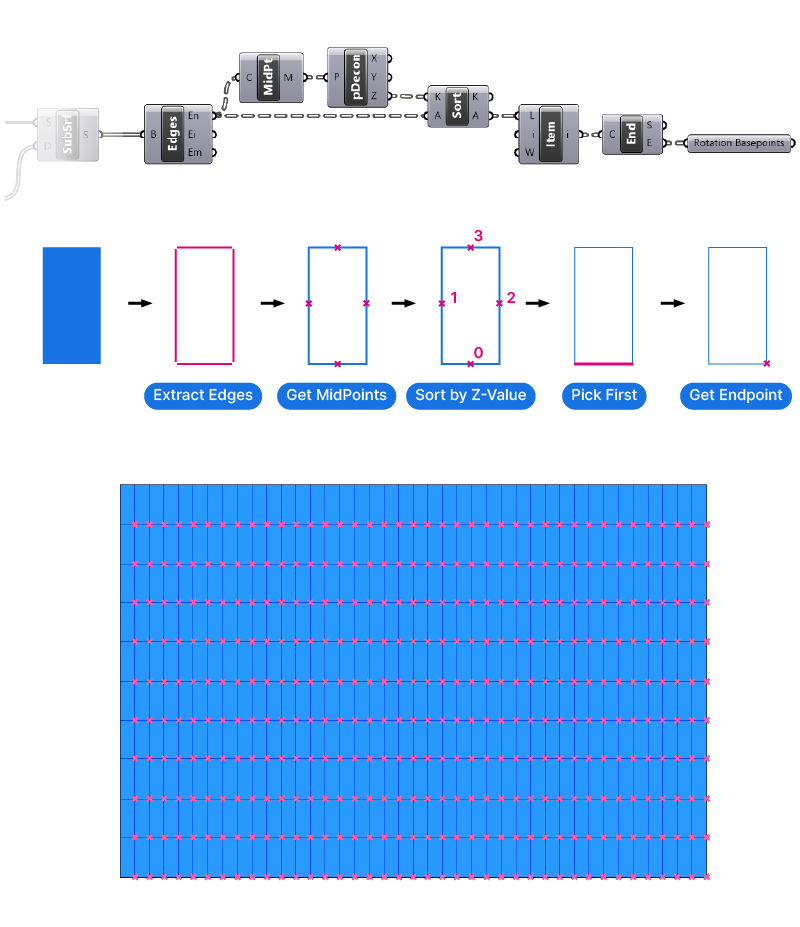
Let’s begin by extracting the edges of each surface with the Edges component.
The Edges component groups the resulting four edge curves in their own dedicated branches.
To get the bottom edge, we need to sort all the edges by their Z-coordinate, and pick the one with the lowest Z- value.
Since curves don’t have a Z coordinate property, we first need to generate a point that represents them, so let’s add a Curve Middle component to get the middle point of each curve.
Now we can use a Deconstruct XYZ component to get to the points’ XYZ coordinates and sort the Z values and the edges in parallel. To do that, we connect the Z-values to the K input, and the edge curves to sort in parallel to the A input.
Since the Sort component always sorts numbers from the smallest to the largest, the curve with the lowest Z-value will be the first in the list. Let’s add a ListItem component and leave the default index input value (I) of 0. That way, we’ll get the first item in the list, which is the bottom curve.
We can simply pick one of the two endpoints of this bottom edge as the rotation point, so let’s add an Endpoints component, which will output the start and endpoint of the curve.
Let’s add a Point container, connect the endpoints, and call it ‘Rotation BasePoints’.
Let’s group these components to keep the script organized.
Rotating the surface panels
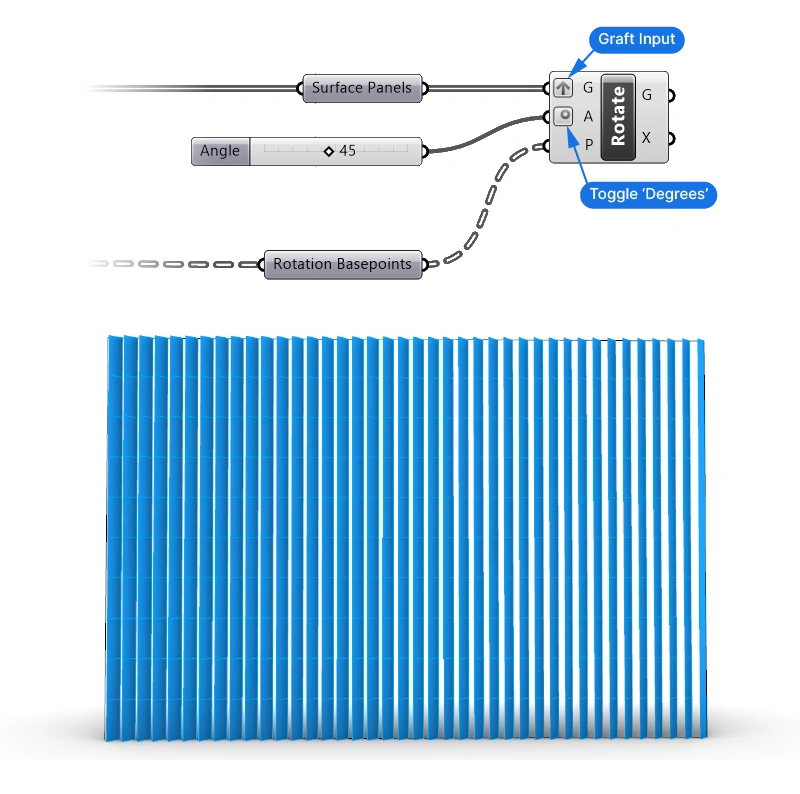
Now we have everything we need to rotate the curve. Let’s add a Rotate component. We’ll pick the one that says ‘Rotate object in a plane’.
The geometry to rotate (G) is our surface panels, and the ‘Rotation BasePoints’ are our rotation planes (P). Make sure to graft the G input, so the data structures match. By providing a point to the rotation plane input instead of an actual plane, Grasshopper will use the default XY-Plane (ground plane) at that point.
We are going to provide the rotation angle in degrees, so let’s right-click on the Angle input of the rotate component and activate the Degree option.
It’s best to test the transformation before we move on to the next step. We can add a number slider with a value of 45 to test if everything works as expected. All panels should rotate 45 degrees.
Let’s turn off the preview of everything we don’t need to see by selecting the components we want to hide, and hitting Ctrl+Q.
Getting the distance to the attractor curve
So far, we’ve applied a single, manually defined rotation angle value to all panels. The next step is to replace it with individual, parametric rotation values for each panel.
We’ll need to calculate the distance from each surface to the closest point on the attractor curve.
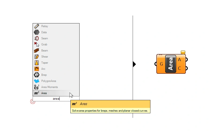
The first step is to generate a point for every surface panel. These are the points we are going to measure the distance to the attractor curve from. Let’s generate it with an Area component. Besides the surface area (A), this component outputs the centroid of each surface in the second output (C).
Now it’s the time to define our attractor geometry!
Let’s start by drawing a curve in Rhino and referencing it to a Curve container. It can be a line or a smooth curve.
Next, we’ll calculate the shortest distance between the surface centerpoints and the attractor curve. We can achieve that with the help of Closest Point components. Let’s double-click onto an empty spot on the Grasshopper canvas and type “CP” into the search bar – CP stands for Closest Point.
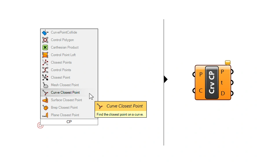
In the results we see all the different kinds of geometries we can use as attractors:
The closest point to a plane, the closest point to a curve, to a Brep, mesh or points.
Let’s add the Curve Closest Point component. We can connect our surface panel centerpoints to the first input P. This are the points to search the closest distance to the curve from.
Let’s connect our referenced attractor curve to the C input – the curve to measure the shortest distance to.
The Curve Closest Point component finds the closest Point on the curve, and then outputs the resulting Closest Point (P), the Curve Parameter at that point, as well as the Distance (D) to that point. The Distance (D) is what we’re looking for in this case.
Tip: We can visualize the distance between each point and the curve by drawing a line between the centerpoints and the closest points output (P) with a Line component.
Remapping the distance to the transformation
The last step to your first attractor curve in Grasshopper is to map the distance values to the rotation.
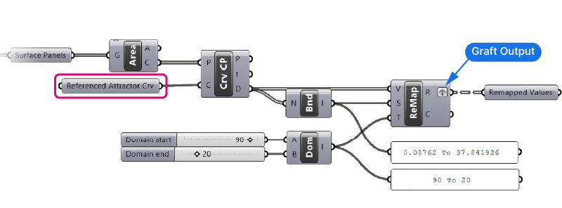
Next let’s add a Remap component to map these distances to a rotation angle.
The Remap component has three inputs:
- V – the values to remap (our distances)
- S – the source domain (minimum and maximum value of our distances)
- T – the target domain (minimum and maximum values of our rotation)
The values to remap are the distances from the surface to the attractor curve. We find them in the Curve Closest Point Distances output D.
Let’s add a Bounds component to generate the source domain from these distance values. And then plug it into the Source domain input.
Lastly, let’s add a Construct Domain component to define our target domain.
Let’s say that our rotation will go from 20 degrees to 90 degrees. We’ll add two number sliders with those values.
The output R of the Remap component now contains the distance values remapped to angle values.
All three outputs: the rotation values, the surfaces to rotate and rotation planes come together in the Rotate component. To make sure the data from all three sources is matched correctly, we need to ensure their data structure is the same.
The rotation basepoints and the surfaces are already grafted, so we need to graft the output of the Remap component as well before connecting it to the Angle input of the rotate component.
Currently the surfaces panels closest to the attractor curve are rotated the least, let’s invert the gradient to fix that.
We can simply switch around our angle inputs of the target domain. The values will now be remapped inversely.
Below the full script and its result:
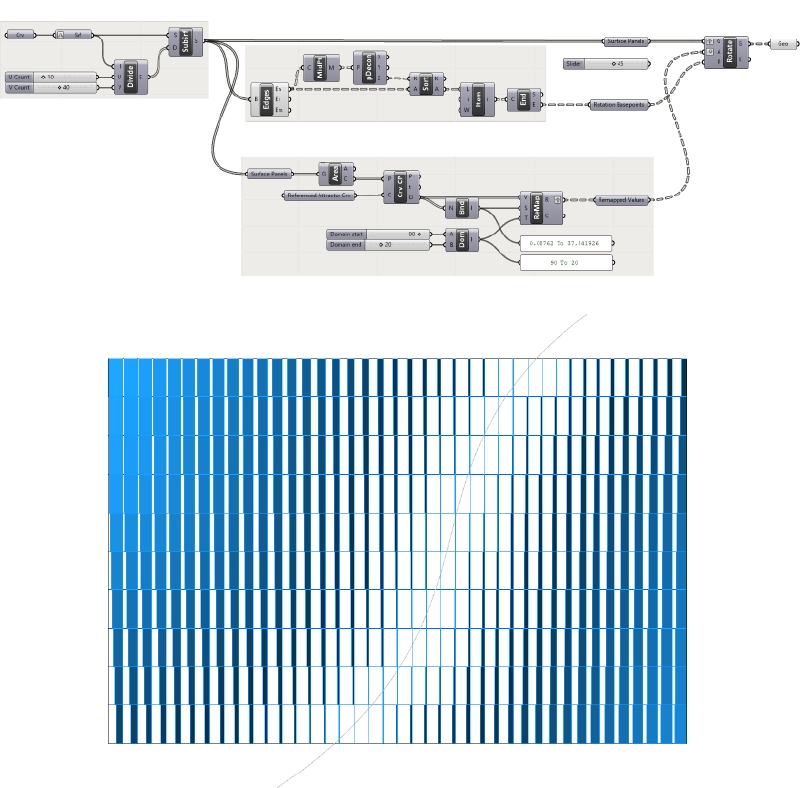
The Bottom Line
So there you have it! We’ve walked through the four steps to create an attractor curve in Grasshopper: setting up a field, defining a transformation, calculating the distance and remapping the distances to the transformation. Along the way, we’ve learned how to use the Closest Point and Remap components.
Experiment with different transformations as well as different attractor geometries and see what kind of results you can achieve!
This is just the beginning of your journey into the world of parametric design using Grasshopper. With these basics under your belt, the possibilities are limitless!
Happy designing!