Creating a sine curve in Grasshopper involves generating a series of incremental values and using the Expression component to run the sine function on them. You can then use the resulting values to either plot the points or move them in the desired direction. The Interpolate component can then be used to create a smooth curve through them.
In this tutorial, I’ll share the technique I’ve found most useful in over a decade of experience as a computational designer, and guide you through the process step-by-step.
Before we jump into Grasshopper, let’s first cover the basics.
Understanding the Sine Function
What is a Sine Function?
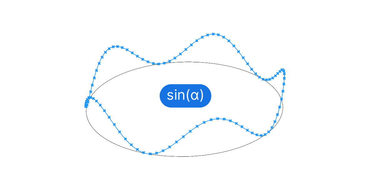
The sine function is a fundamental concept in trigonometry that describes the relationship between the sides of a right-angled triangle in relation to one of its angles. In its simplest form, the sine function is written as:
y=sin(α)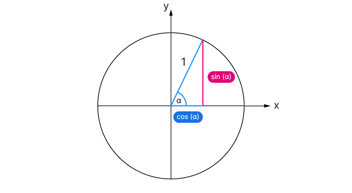
Here, α (alpha) represents the angle in radians (fractions of π), and sin(α) equals the length of the side of the triangle opposite the angle.
The true elegance of the sine function becomes visible when we plot it on a Cartesian coordinate system. Instead of limiting α to angles within a unit circle, we can extend it to any range of positive and negative numbers. This extension transforms the sine function into a continuous, visually appealing wave-like curve.
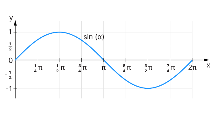
When designing with sine curves, the parameter x doesn’t have to be restricted to radians; it can be any real number. This is key — it’s what allows us to generate a sine curve in many different ways inside Grasshopper.
Let’s learn how to create a basic sine curve setup in Grasshopper next!
Basic Sine Curve Setup in Grasshopper
The basic setup for creating a sine curve in Grasshopper is to generate a series of equally spaced incremental values that represent the x values, and using the sin(x) formula to generate the matching y values to create the wave.
Follow these steps to create a basic sine curve:
Generate a Series of Numbers
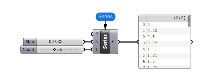
Add a Series component to generate a sequence of numbers. This will represent the x-coordinates of your sine curve.
The Step (N) controls the spacing of the sample points. Choose a small value (e.g., 0.25) to ensure the curve appears smooth.
The Count (C) will control the number of sample points and thereby the length of the resulting wave.
Create Points
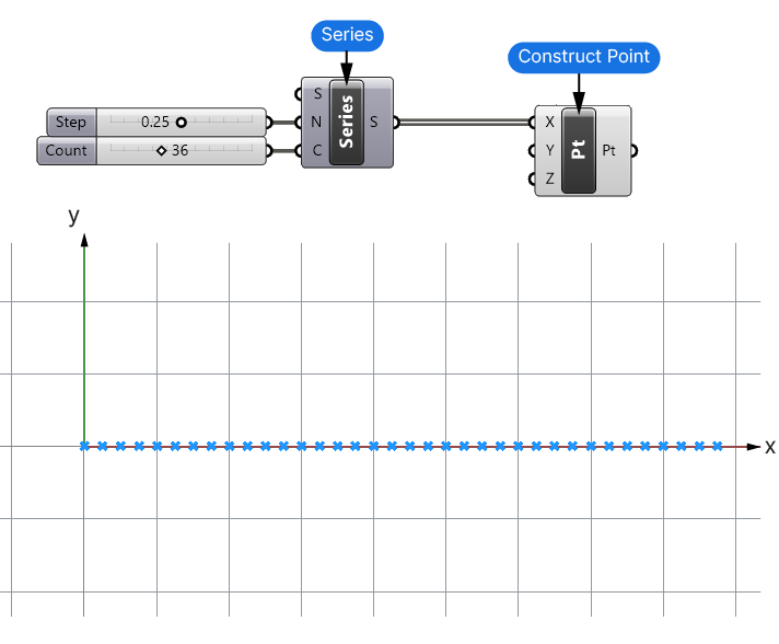
Use a Construct Point component to generate points from the number series. Connect the output of the Series component to the X-coordinate input of the Construct Point component.
This will generate an array of points in the viewport along the x-axis.
Apply the Sine Function
Insert an Expression component to apply the sine function to the x-coordinates to create the y-coordinates.
Enter the expression sin(x) where x is the output from the Series component.
This step will generate the y-coordinates for each value x based on the sine function. Then connect the output to the Y-coordinate input of the Construct Point component.
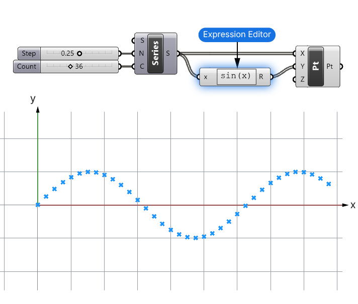
The points will now describe the sine wave form!
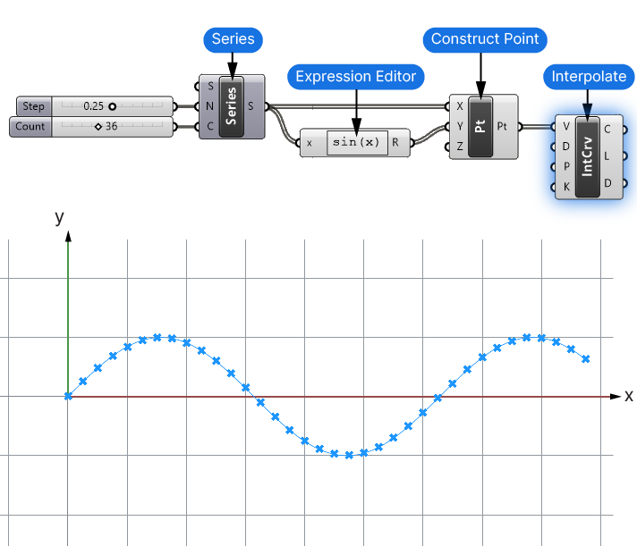
Connect the Points with an Interpolated Curve
To create a smooth curve from the points, use the Interpolate component.
Connect the output of the Construct Point component to the Vertices input of the Interpolate component.
In this example we’ve created the sine curve using just x and y coordinate values. We’ve also used the simplest form of the sine function: sin(x).
Without any additional parameters, the sine function will always return values that range from -1 to 1, as the output above shows. In addition, we can’t control the frequency of the wave.
To use the sine function effectively in our designs, we’ll need more control. Let’s learn how to get that next!
Controlling the Sine Curve: Amplitude, Shift and Frequency
To use the sine curve to full effect in our designs, we need more control over its shape and trajectory. There are four parameters we can add to the default y = sin(x) function to get more control. Here is the formula:
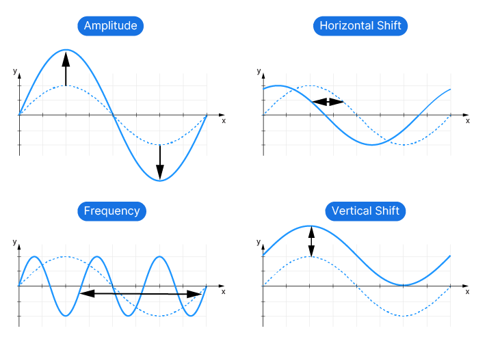
y=Asin(Bx+C)+DHere’s what each parameter represents:
- A: Amplitude. It controls the height of the wave. Larger values of A make the wave taller, while smaller values make it shorter.
- B: Frequency. It controls the frequency of the wave. Larger values of B make the wave cycles more frequent (compress the wave), while smaller values spread out the cycles (stretch the wave).
- C: Horizontal (Phase) shift. It controls the horizontal shift of the wave. Positive values of C shift the wave to the left, while negative values shift it to the right.
- D: Vertical shift. It controls the vertical displacement of the wave. Positive values of D move the wave up, while negative values move it down.
Advanced Example: Sine Curve Along a Circle
Let’s learn how to apply the above formula. Here’s our design goal: we have a circle and we want to create a sine curve that neatly connects on its ends, forming a smooth, continuous sine curve.

Script Setup
Let’s start with the guide curve. I’ll reference a circle with a radius of 30 units from Rhino to a Curve container to start things off.
To apply the sine function, we need a list of incremental numbers that act as our x values. Since we have a circle we can’t use the x,y,z coordinates this time. Instead, we’ll use curve parameters along the curve.
To generate equally spaced points along the curve, we’ll use the Divide Curve component.
We’ll need both the Point (P) output of the Divide Curve component, as well as the Curve parameter (t) values. These numerical values describe the position on the curve and will serve as our x values.
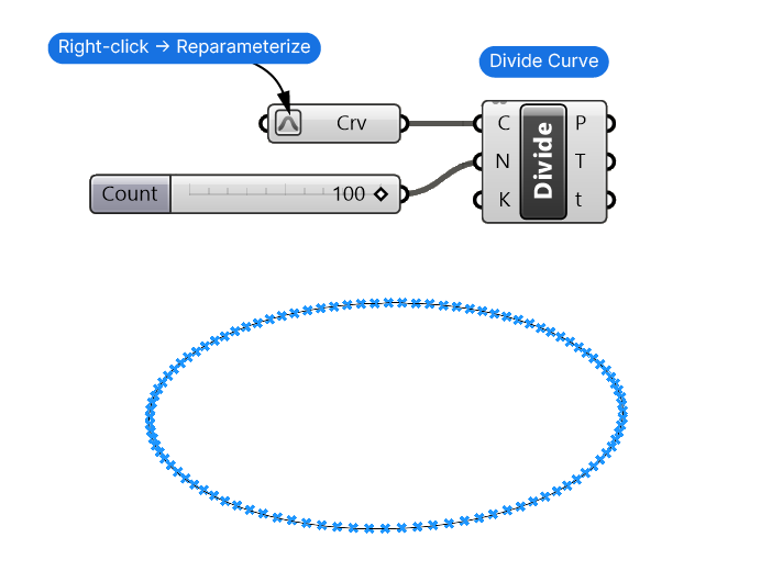
Now by default, the curve parameter (t) values can be any kind of number – so let’s right-click on the curve container and select ‘Reparameterize‘ to ensure the values range from 0 to 1. It’s important to control the range since the sine function will always calculate using the Radians range which goes from 0 to 2π (roughly 6.28).
If you leave these values up to chance you have no control over the sine curve.
Preparing the incremental values for the sine function
To ensure that the sine curve we create forms a complete, clean loop, we need to ensure that we are working with a full sequence of the sine curve: the valley as well as the mountain.
To achieve that we’re going to remap the curve parameter t values to 0 to 2π — a full rotation around the unit circle. Let’s add a Remap component, connect the Curve Parameter (t) output to the Values to Remap (V) input, and a Pi component to the Target Domain (T) input.
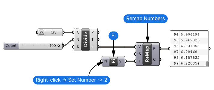
Since π only represents half a sine curve, let’s right-click on the Factor (N) input, go to Set Number, enter 2, and click Commit changes.
We can leave the Source Domain (S) untouched since it ranges from 0 to 1 by default.
If we check the remapped values, we see that the numbers now range from 0 to about 6.28 — the numerical equivalent of a full sine rotation.
Now we are ready to feed the values through the sine function.
Adding the sine function
Let’s add an Expression Editor and type in the formula sin(x). We’ll connect the Remapped Numbers (R) to the x input.
The Expression Editor output values now represent the sine curve, but how do we use them to create the sine curve?
We can simply move the division points we created earlier vertically by the amount specified by the values. To do that we need both a Move component and a Unit Z component. The sine(x) output will be the input for the Unit Z component, creating vertically vectors of the length specified by the sine(x) values.
The Move component will then move the original division points by the resulting vectors.
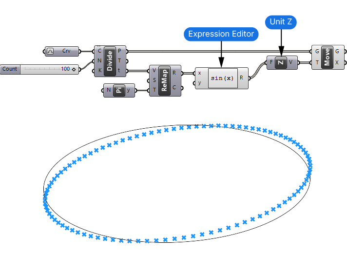
Finally let’s add an Interpolate (IntCrv) component to create a smooth NURBS curve from the resulting points.
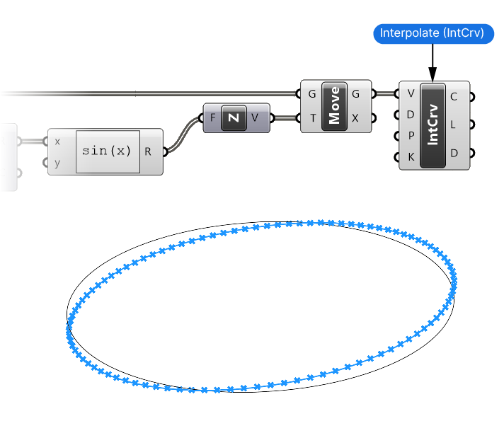
Once everything is connected, we get what looks like a tilted circle. That’s because we remapped our “x-values” to exactly one rotation. The tilted curve represents the upward portion of the sine curve on one side and the lower portion on the other!
Extending the sine function
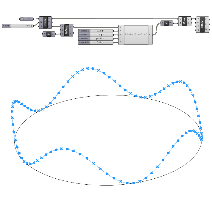
Let’s modify the sine function in the Expression Editor to get more control. Change
y=sin(x) to y=A*sin(B*x+C)+DSince we’re adding four additional parameters to the formula, make sure to zoom up close to the inputs of the Expression Editor, and click the small plus signs to add four more inputs. Name them to match the variable names in our formula: A,B,C, and D.
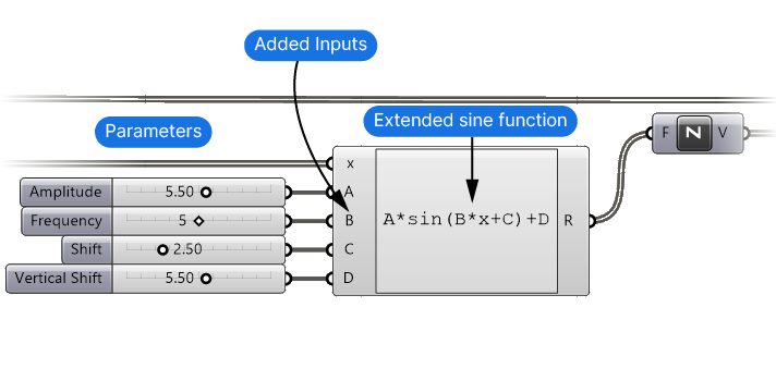
Next let’s add Number Sliders for each, starting with input A. Create a Number Slider with a double-digit precision and a range from 0 to 10. This value will control the Amplitude. The number we enter here equals the height of the valley and hill. In other words half the total height of the generated sine curve.
The parameter B represents the multiplier for the number of waves we’ll have along the curve. Since we want to connect the sine curve cleanly in a loop, let’s only use integer numbers without any decimals.
Let’s add two more Number Sliders with a range of 0 to 10 and double digit precision. The parameter C will shift the wave starting point along the curve, and parameter D control the height location of the entire curve.
Let’s set the height location (D) value to the same as the amplitude. That way the sine curve will sit neatly on top of our referenced curve.
And that’s it! That’s how you create a sine curve while keeping full control over the parameters that matter for design applications!
Tweak the sliders and see what you can come up with!
Note: Increase the number of Division Points if your interpolated curve looks choppy. Having enough sample points is crucial for a smooth curve.
Concluding thoughts
Understanding and controlling parameters like amplitude, frequency, phase shift, and vertical shift are the key to controlling a sine curve precisely in Grasshopper. While it might be tempting to simply scale or deform a generic sine curve, learning these parameters will make your life easier and your scripts more robust.
Happy designing!