Step into the world of advanced parametric design with our guide on the multiple curve attractor effect in Grasshopper. This tutorial will take you through the essentials of creating complex and responsive designs using multiple attractors. Perfect for both beginners and experienced users, we’ll break down the process into simple, manageable steps to help you master this powerful feature and bring your designs to life.
Let’s get started!
The Logic Behind Multiple Curve Attractors in Grasshopper
Before we dive into which Grasshopper components to use, like with all scripts, it’s important to understand the logic behind the multiple curve attractor effect.
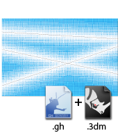
Like all attractor effects, the starting point for the multiple curve attractor script is a grid of objects, which I’ll refer to as a “field”. Elements in this ‘field’ react to multiple curves by modulating the extent of a geometric transformation. The outcome is a visual effect of a gradient or smooth transition.
The key to the effect is the ‘modulation’ part. How do we control which elements are transformed, and by how much? In contrast to single attractor geometries, where the transformation is driven by the distance to the geometry, with multiple attractor curves, we calculate the closest distance to any of these curves.
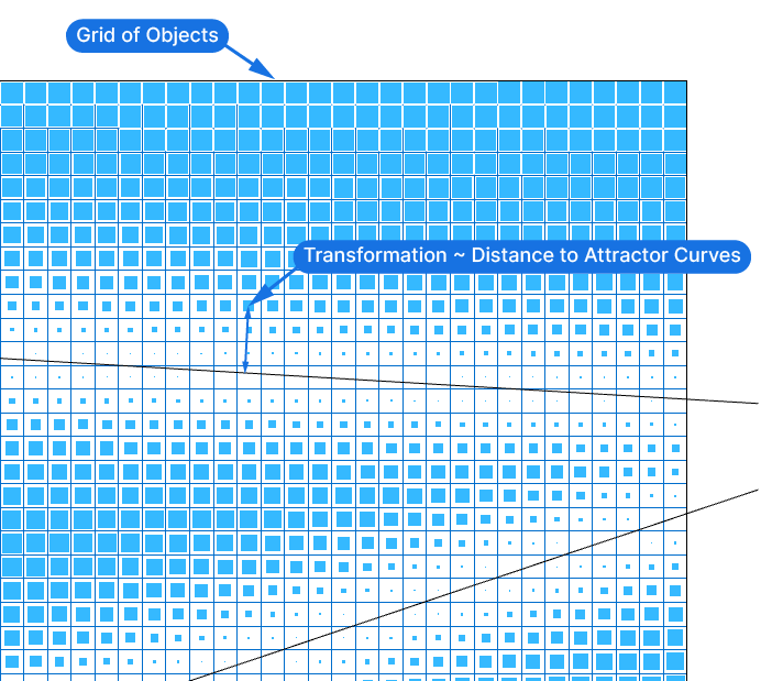
This means that from each element in the field, we’ll need to calculate the closest distance to each one of the attractor curves, and then finally pick the closest distance.
Once we have the closest distances for all the elements, we can remap the distance values to a geometric transformation we define. This could be something as simple as scaling or rotation, or a more complex series of geometric operations.

In summary, creating a multiple curve attractor effect can be done in four steps:
- Step 1: Create a field of objects
- Step 2: Set up a geometric transformation for the objects in the field (for example scaling)
- Step 3: Calculate the distance to the closest attractor curve
- Step 4: Remap the resulting distances to transformation values
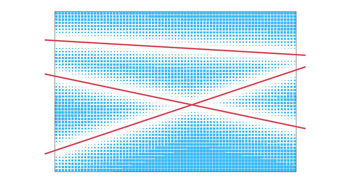
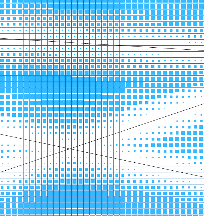
Once set up, we can add as many attractor curves as we want, and the grid or field will react to all attractors as shown below!
Let’s learn how this attractor curve logic can be broken down into components inside Grasshopper!
Multiple Curve Attractors – Step-by-Step Tutorial
Step 1: Creating a grid of objects
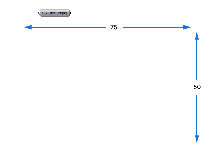
Let’s start by setting up a base grid that we’ll use our attractor effect on. We’ll draw a rectangle of 50 by 75 units in Rhino, and reference it to a Curve container inside Grasshopper.
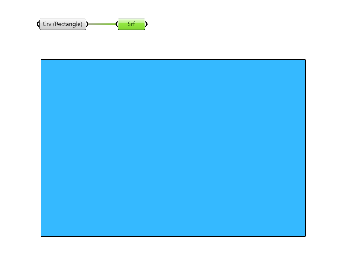
A simple way to create a grid within a curve, is to first convert it to a surface, and then dividing the surface’s domain to extract a series of subsurfaces. It will be clear in a second:
Start by adding a Surface container component to your script, and connect the referenced curve to it. Since the curve is a closed, planar rectangle, the surface container will automatically convert it into a surface.
Dividing the Surface Domain
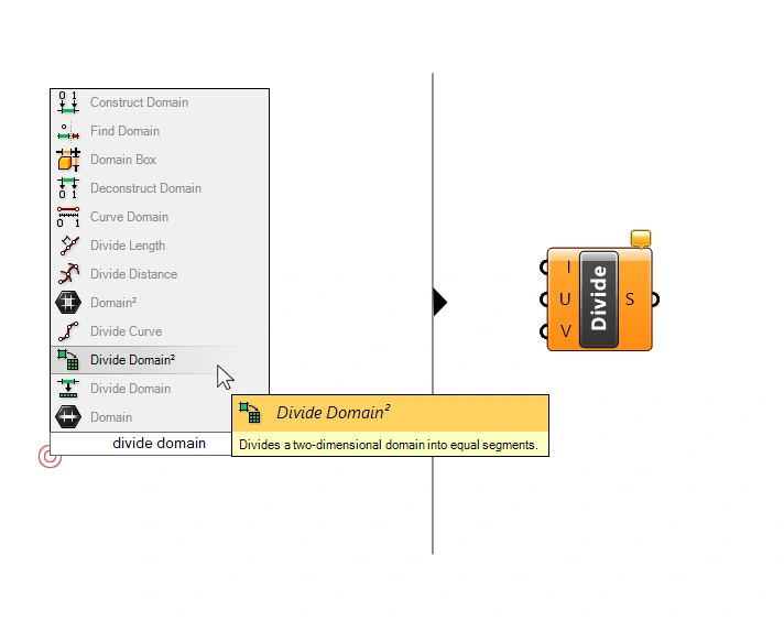
Next we’ll need two components: the Divide Domain² (Divide) component and the Isotrim (SubSrf) component. Type their respective names into the component search bar to add them to your script.
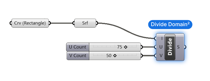
Let’s start with the Divide Domain² component. Type ‘Divide Domain‘ into the component search bar and select the one with the ² symbol to add it to your script.
We connect the Surface to the Domain (I) input. This provides the Divide Domain² component with the surface domain to divide. Since the domain of a surface is two-dimensional (U-and V-directions), we get to choose the number of subdivisions for both the U and V- direction in the U-Count (U) and V-Count (V) inputs. In other words, the vertical and horizontal divisions of the surface.
Since our rectangle is 50 by 75 units large, let’s divide the U and V domain by the same numbers to get a grid of 1 x 1 units. Use two Number Sliders, and make sure the U and V values match your rectangle orientation, to avoid a distorted grid.
Great, so we now have a set of two-dimensional domains that describe the squares on our surface. But for now they are just numbers. That’s where the Isotrim (SubSrf) component comes in.
Extracting the Sub-Surfaces using the Divided Domains
Type ‘Isotrim‘ into the component search bar and select it add it to your script.
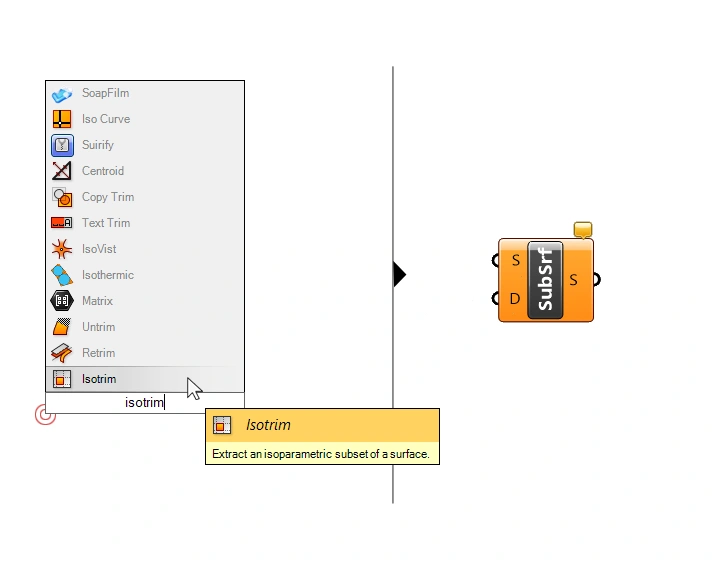
Connect the Surface to the Surface (S) input, and the Divide Domain² output to the Domain (D) input.
The Isotrim (SubSrf) component outputs all the sub-surfaces described by the domains we connected.
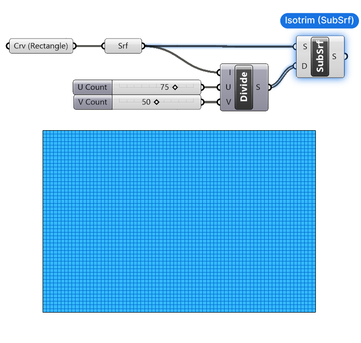
Great! We have successfully created our grid of objects!
Step 2: Set up a geometric transformation for the objects in the grid
Any attractor effect only becomes readable through the transformation of the objects in the grid we define. This transformation can be anything from a simple operation like scaling, rotating, all the way to complex chains of transformations. The only requirement is that the transformation can be driven by a single numerical input in the end.
Since the focus of this Grasshopper tutorial is in the multiple curve attractor algorithm, we’ll use a basic scaling command for the transformation. Let’s set it up!
Let’s add a Scale component.
The Scale component has three inputs:
- the Geometry (G) to scale
- the Center of scaling (C)
- the Scaling Factor (F)
The geometry to scale is our grid of surfaces, let’s go ahead and connect them. Next we need to specify the center of scaling. We want to scale each element in place, so let’s add an Area component, to generate the centerpoint of each surface. The Area component outputs the area of the surfaces, but in the second output “Centroid” (C) it provides us with the center points of each.
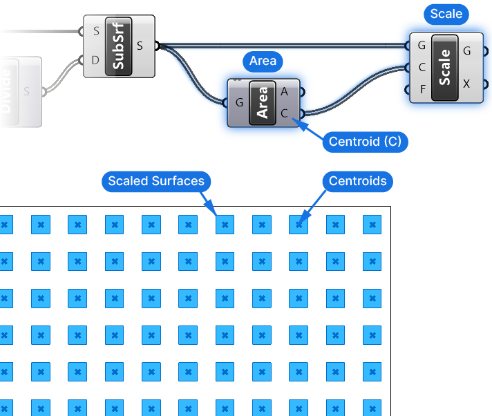
Exactly what we need! Let’s connect it to the Center of Scaling (C) input of the Scale component.
The last input to define is the Scaling Factor (F). This is the value we’ll define based on the attractor curves, so let’s leave it at its default value of 0.50 for now.
Alright! The transformation is set up, and we already have a reference point for each surface in the grid. Next we’ll find the distance to the closest attractor curve!
Step 3: Calculate the distance to the closest attractor curve
Now we’ll need some attractor curves. So let’s go ahead and draw a few curves that run across the grid, and reference them to a new curve container component. I’ll right-click on the component and name it ‘Attractor Curves’ for clarity.
To find the closest point to a curve, we can use the Curve Closest Point (Crv CP) component. Let’s add the component by double-clicking on an empty spot on the canvas, and typing “crv cp”, and selecting the first result.
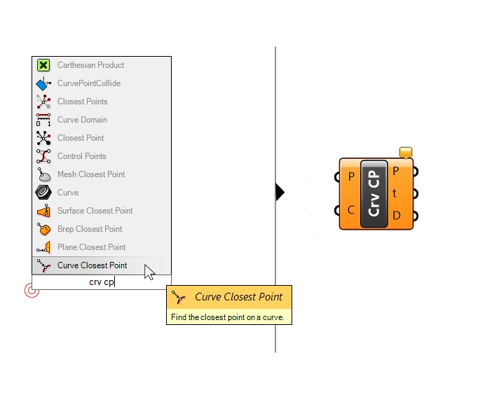
As the name suggests, the component will find the closest point on a curve (C) from a point (P) we provide. Besides the closest Point (P) itself, the component also outputs the Distance (D) to this closest point – that’s what we’re looking for.
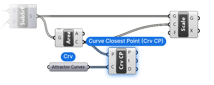
Let’s go ahead and connect both the Centerpoints and the Attractor Curves to the Curve Closest Point (Crv CP) component.
Managing the Data Structures
Here’s where we need to pay special attention to the data structure. As it stands, we have connected two lists of data. The points come in a list, and the curves as well.
Whenever two data streams containing lists are matched in a component, Grasshopper will match the first item of the first list with the first item of the second list, and so on. Once the second list runs out of elements, all remaining items of list one will be connected to the last valid item of list two. In practical terms, all except for the two points will measure the closest distance to the third curve in our list.
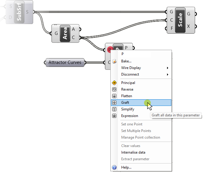
But for our algorithm to work, we need to measure the distance to each curve, and then select the closest one. To achieve that, all we need to do is graft the Point (P) input. To do so, right-click on the Points (P) input and select ‘Graft’.
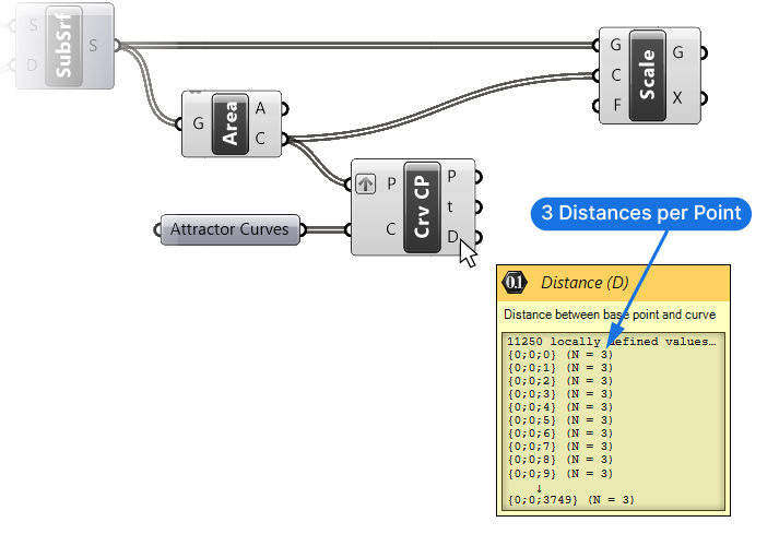
A quick hover over the Distance (D) output shows that we now get three distance values for each point. Perfect!
Getting the Closest Distance
Now let’s sort these distances. Add a Sort List component, and connect the Distance (D) values to the Keys (K) input. The Sorted Keys (K) output contains the distances, sorted from smallest to largest. Let’s pick the smallest distance by picking the first item in the list with the List Item component.
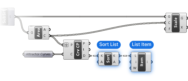
Add a List Item component, and connect the Sorted Keys (K) to the List (L) input. The List Item component comes with a default index (i) of 0, which is the first item in a list, so no further inputs are necessary!
Fantastic! We’re close! We’ve found the closest distance to the attractor curves. The last step is to remap these distance values to a target transformation.
Step 4: Remap the closest distances to transformation values
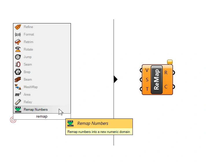
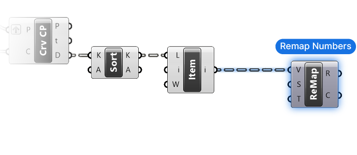
We’ve come to the crucial step of any attractor algorithm: Remapping the distances to the transformation. Let’s begin by adding the Remap Numbers (ReMap) component.
The Remap Numbers component has three inputs:
- The Values (V) to remap
- The Source Domain (S) of the values to remap
- The Target Domain (T) to remap the values to
We already have the values, which is our distances, so let’s go ahead and connect them to the Values to Remap (V) input.
Generating the Source Domain
Next we need the Source Domain (S). Why do we need it? Because to remap values we need to know where to remap them from. In our case, the Source Domain ranges from the smallest distance, meaning the surfaces closest to an attractor curve, to the largest distance, or the surface farthest away from the attractor curves.
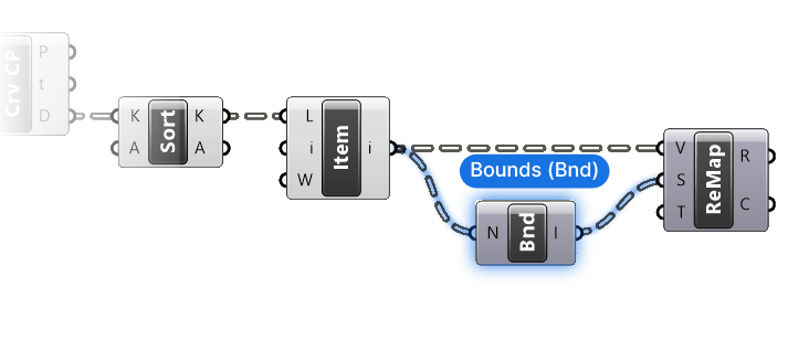
Luckily we don’t have to construct this domain manually, we can extract the so-called ‘Bounds’ of a list of numbers (meaning the smallest and largest numbers) with a component called … Bounds!
Let’s add it to our script and connect the distances. We can also already connect the output to the Source Domain (S) input of the Remap component.
Now we need the bounds of all the distances, but currently the distances are stored in separate data branches, one for each point. So let’s go ahead and ‘flatten’ the List Item output containing all our distances.
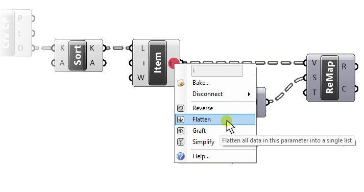
Perfect.
The third input asks for the Target Domain (T). Let’s leave it at its default of 0 to 1. This means that the shortest distance will be remapped to a value (or scale) of 0 and the largest to a scale of 1.
Let’s test this by connecting the Mapped (R) values output to the Scaling Factor (F) input of the Scale component. Low and behold we see a first version of our effect!
Modulating the Gradient Fall-off with the Graphmapper
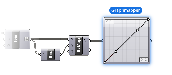
The grid is reacting to the attractor curves, but the effect is hard to read. To get more control over the fall-off of the gradient, we can use the Graphmapper component.
Type ‘Graphmapper‘ into the component search bar to add it to your script.
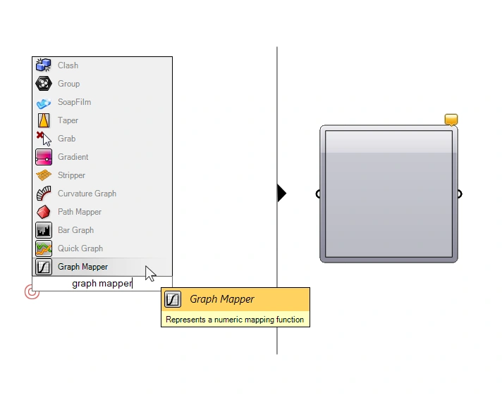
By default, the Graphmapper is just an empty gray panel with a single in-and output. The Graphmapper allows us to modulate a list of values through a mathematical graph. This sounds quite abstract, but it’s really quite simple: To start, right-click on the component, and go to Graph types, and select ‘Bezier‘.
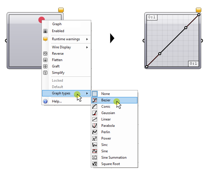
The component canvas now comes to life and we see a linear, diagonal graph. Click-and-drag on the dots in the graph to start modulating the graph curve. This is how we are going to control the fall-off of our attractor effect.
Let’s connect our remapped values to the Graphmapper input. As shown by the numbers in the corners, the Graphmapper modulates numbers within the range of 0 to 1. This matches exactly with the default Target Domain of the Remap component.
Remapping the Modulates Values to our Target Domain
Now that we have the modulated values, we can add a second Remap component and map these values to our actual target transformation.
Connect the Graphmapper output to the Values (V) input. This time we don’t need to connect a Source Domain, since the default of 0 to 1 works perfectly fine.
To define our own Target Domain (T), we’ll use a Construct Domain component.
Add two Number Sliders with a values of 0.05 for the smallest scale and a value of 1.00 for the largest. (We don’t want to scale all the way to 0 as that will throw an error).
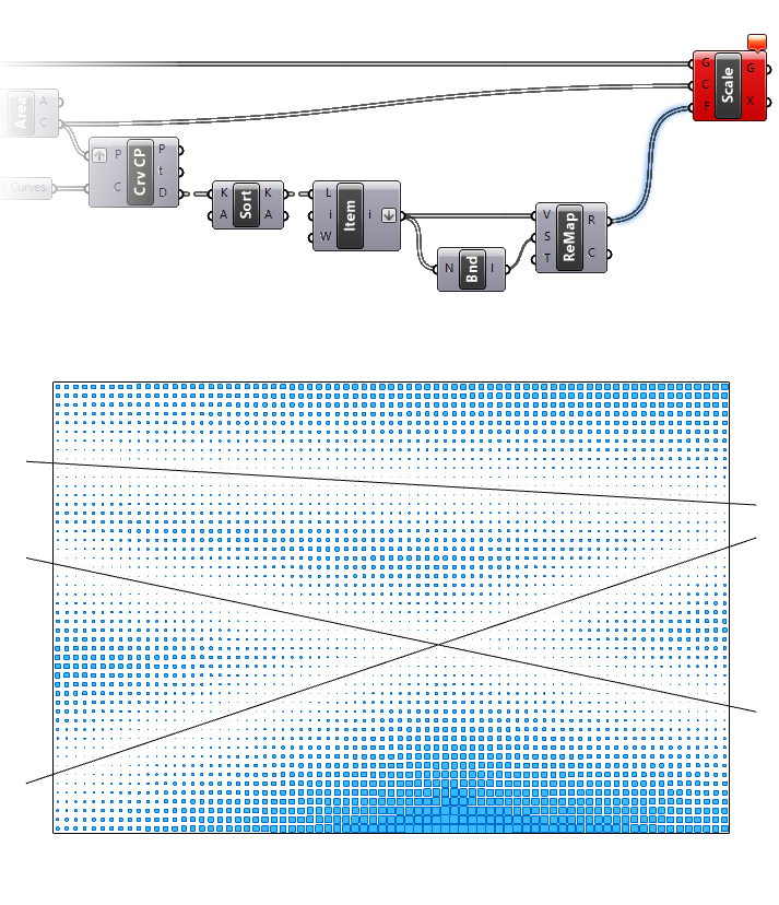
Finally connect this constructed domain to the Target Domain (T) input, and then the resulting remapped values (R) to the Scaling Factor (F) input of the scale component.
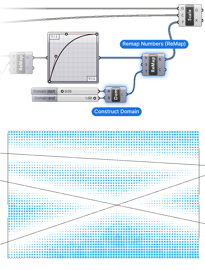
Now that we see the result of our modulated effect, we can go to the Graphmapper and tweak the graph to get just the fall-off effect we want.
And there you have it! You’ve just created a multiple curve attractor effect! Congrats!
See the full script below:
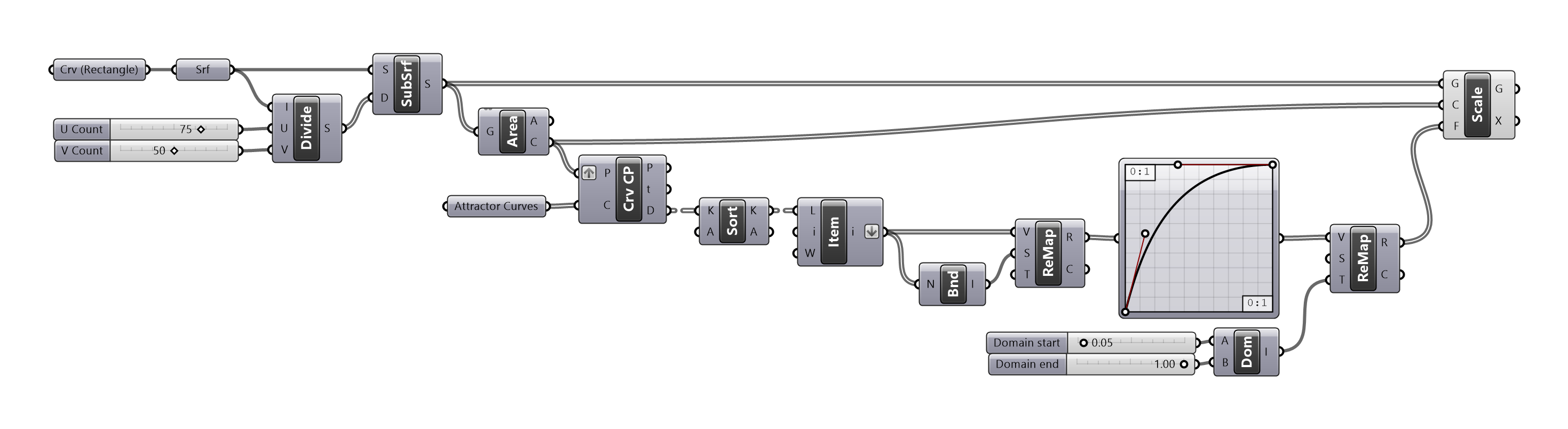
Multiple Curve Attractors – Final thoughts
While the multiple curve attractor effect in Grasshopper is largely based on the same logic as a single curve attractor, it does require the extra step of calculating the distance to all attractor curves and finding the distance to the closest one.
I hope you found this tutorial helpful!
If you are a designer interested in mastering Grasshopper, check out my online course Grasshopper Pro – it’s a comprehensive course that teaches you all the techniques used in a professional design practices.
Happy designing!