The Galapagos component in Grasshopper stands out with its bright pink color, and for good reason: it’s much more than a simple component. With it, we unlock the ability to find the optimal solution given any number of variable parameters. Now this may sound very abstract, but I’ve made it my goal for this article to explain what it does and how to use it in your scripts in the most clear and straight-forward way possible.
At the end I’ll show you a practical example of how to use this powerful component.
Let’s dive in!

Galapagos 101: A Primer
Let’s start with the name of the component. The unique name is not by chance – it hints at the Galapagos islands, which inspired Charles Darwin to come up with the theory of evolution. The animals that Darwin encountered on the Galapagos Islands would help inform his theory of evolution by natural selection: “one general law, leading to the advancement of all organic beings, namely, multiply, vary, let the strongest live and the weakest die”.
You may wonder how this ties back to Grasshopper! Well, the Galapagos component uses a similar “evolutionary” approach to finding the optimal set of parameters. For this optimization to make sense, we need to specify a ‘fitness’, in other words, something that we are trying to optimize for. For example, one species of birds on the Galapagos islands evolved to have longer beak to better reach the seeds of the local plants. In this case the optimization was to get to food more easily.
‘Fitness’ in Galapagos
When it comes to defining fitness in Galapagos, we can define the fitness much more concretely, with a number.
Once we have a number to define the fitness, there are two ways that we can optimize it for: we can optimize for the number to be as large as possible, for example to get as many seeds as possible, or as small as possible, like to pick as few of the poisonous seeds as possible.
As we’ll see once we jump into the Galapagos interface, we need to define whether we want to optimize the fitness for the maximum or minimum.
You may wonder what the parameters are that the component will use to find the optimal solution. The answer is simply – good old Number Sliders! We get to define exactly which Number Sliders we want Galapagos to play around with to get to the best possible fitness.
Once we’ve defined the fitness and the parameters to modify, the Galapagos component will do the rest. It will use one of two algorithms to generate random parameter value sets and compare the resulting fitness values to each other.
The more variation it tests, the more ‘good’ solutions Galapagos finds, and it keeps track of the best solutions with the highest fitness in a kind of scoreboard.
This process is why it’s called the evolutionary solver: starting with random parameter sets, the algorithm gradually learns to adjust these parameters, thereby improving fitness and, consequently, the quality of the solutions.
Naturally, at some point there are no better solutions to be found, or the improvements are only minimal – the results plateau.
Before we explore the application example, let’s discuss when it makes sense to use Galapagos for ‘evolutionary solving’.
The Galapagos Component Interface
How to add the Galapagos component
Let’s start by adding the Galapagos component to the Grasshopper canvas. It’s located in the ‘Params’ component tab, on the far right, grouped under ‘Util’. The component icon looks like two cells.
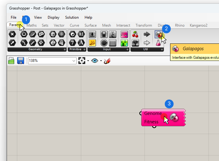
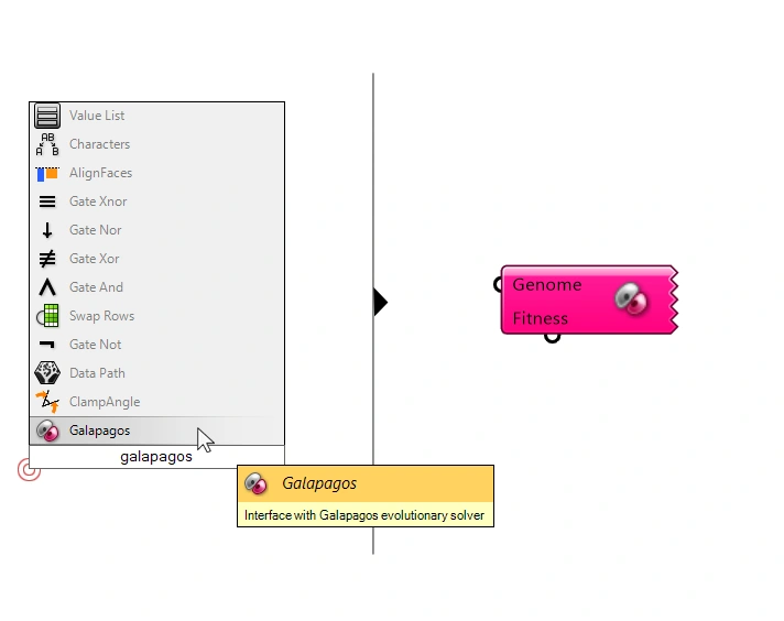
To add it using the component search bar instead, double-click anywhere on the Grasshopper canvas, type “galapagos” and select the first result.
The first thing that you’ll notice, besides the outrageously pink color, is that instead of the normal input and and output on the left and right, the component has an input on the left but another input on the bottom!
The two inputs are easily explained:
- the left-hand input is where we’ll connect all the parameters that we want Galapagos to tweak to find our optimal solution. We can connect any number of Number Sliders we want, but keep in mind that the more parameters you add, the longer the ‘solving’ will take.
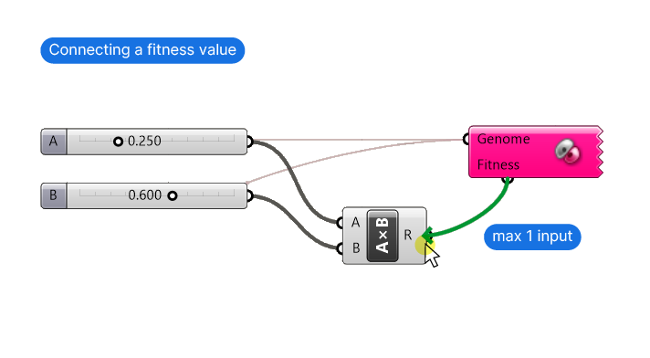
- The input facing downwards is where we can define the fitness: the number that expresses the quality of the solution. We can only define a single number as fitness. This is why we need to carefully think of how to construct this fitness – more on that in the application example coming up.
How to create connections to the Galapagos component
Beyond the strikingly different look, and the unusual input connectors, creating connections to the Galapagos component is also different. If we try to plug anything to either of the two inputs, the wire will simply not ‘stick’.
To create a connection, we need to start creating the connection from the Galapagos component input itself, and drag it ‘backwards’ to any Number Sliders we want to define as parameters. You’ll see a pink connection wire appear with an arrow.
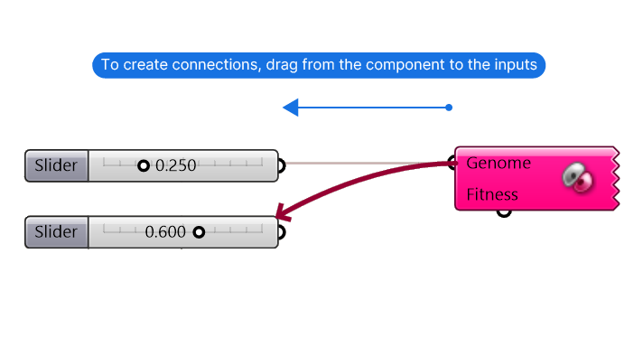
To add multiple inputs, hold down ‘Shift’, just like you would when adding multiple connections to the same input.
We can only connect Number Sliders or the so-called ‘Gene Pool’ component, which is effectively a bundle of Number Sliders with the same ranges packed into a component.
To connect the ‘fitness’ parameter, just like with the parameter inputs, we have to start creating the connection from the Galapagos component and drag it to the number output that defines the fitness. This connection will be green. We can only connect outputs that represent a single numerical value.
In the example below, the output of the Multiplication component is a number, which is why we are able to create the connection.
Now that everything is connected, we can go ahead and fire up the solver. Double-click on the component to open up the Galapagos interface.
The Solver Interface
A window with three tabs opens:
- Options
- Solvers
- Record
The Options tab
On the default Options tab, we see a number of parameters on the left and recommended readings on evolutionary solvers on the right.
The single most important setting on this tab is the fitness. We need to specify whether Galapagos should optimize the number we chose to represent the fitness towards a maximum or a minimum.
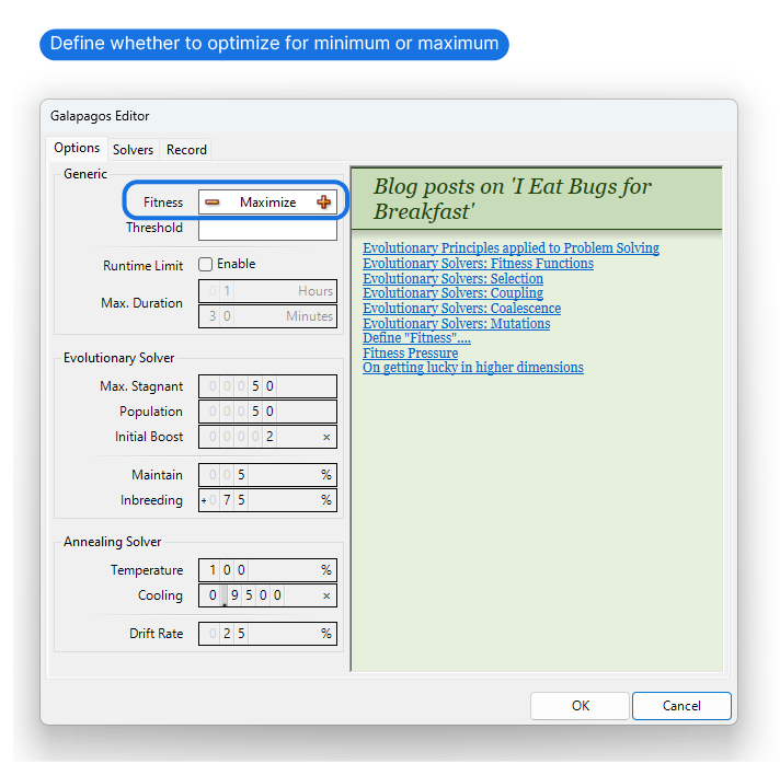
For 99.9% of practical applications, all the other settings on this tab are just fine.
The Solver tab
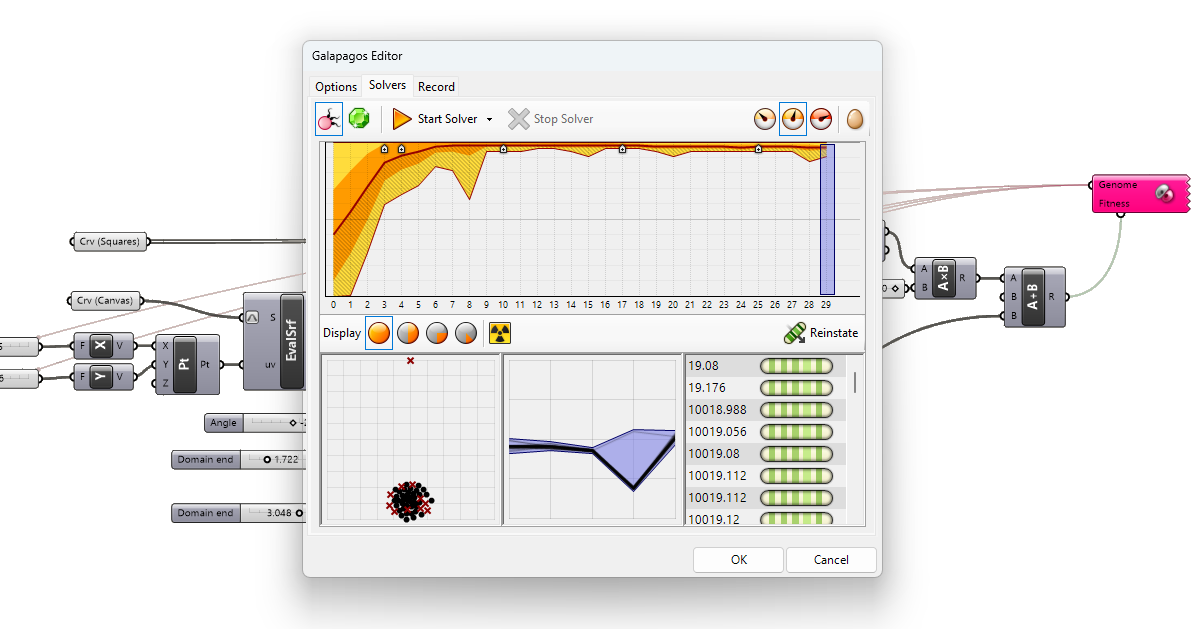
Next, switch to the ‘Solver’ tab. This is where the magic happens!
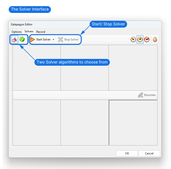
The first two icons on the left allow us to choose the algorithm we want to use for the solving. While one or the other may be better suited for certain tasks, they lead to very similar results.
The algorithms are:
- Evolutionary Solver
- Simulated Annealing Solver
Then, we can go ahead and hit ‘Solve’!
Galapagos will now start playing around with the parameters (“Genomes”) we connected. It will test randomized parameter combinations, and the fitness resulting from them will guide Galapagos to get closer and closer to the maximum or minimum fitness possible with the given parameters.
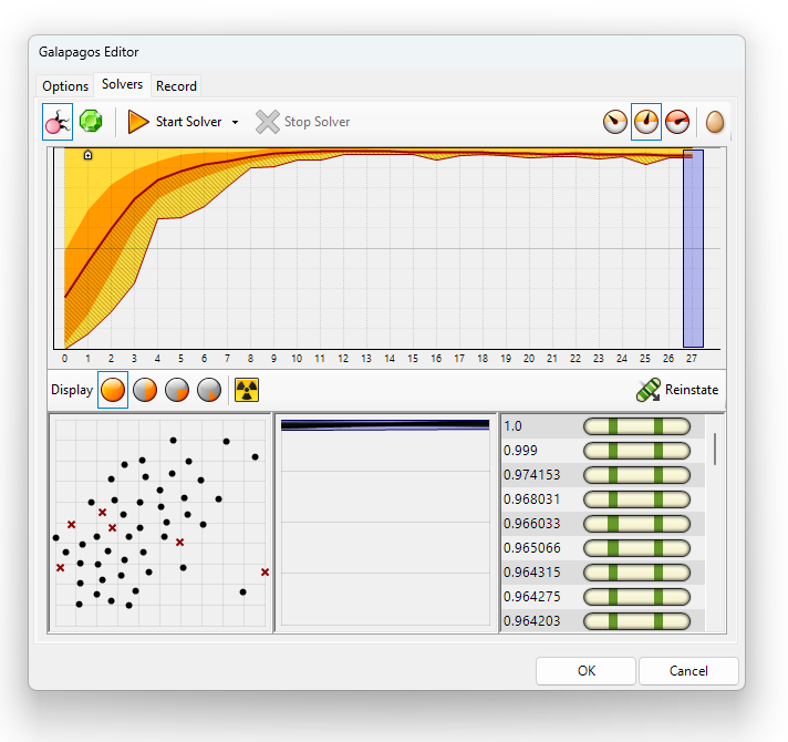
While it’s computing, we get fancy graphs displaying the progression of the optimization. The main window to observe is on the bottom right. The values displayed next to the greenish “Genomes” or simply parameter combinations are the fitness result of the calculations. They are ranked by fitness. Since we chose ‘Maximum’ as the fitness optimization, the largest numbers are shown on top.
Once the algorithm fails to improve the best variation, the solver will stop. Alternatively stop the solver anytime you are happy with the result, by clicking “Stop Solver” to interrupt the solver.
Now while all of this is going on, we can see how the Number Slider values are being tweaked in the background and we also get to see the current best genomes live in our Rhino viewport.
We can choose whether to show each and every genome while the algorithm is running, the better ones or just the best ones, by using the three orange/white speedometer icons on the top right.
Evaluating the Results
Once the solver has stopped running, we can evaluate the results. Usually the best fitness will be the best solution, but we can check out the runner-ups: By selecting the genomes in the bottom right window and clicking “Reinstate“, Galapagos will send the selected Genome parameters to the Grasshopper script and we get to see the result in the viewport.
In our very basic example, we used the multiple of the two Number Sliders as the fitness, and the two sliders as the parameters. Galapagos correctly found that setting both values to 1.000 will lead to the largest value.
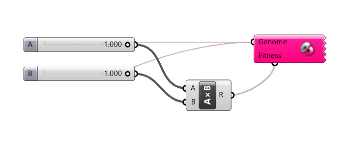
Now be careful, once you click OK and close the Galapagos window, the chosen parameters will be set on the Number Sliders, but you lose all the information about the other genomes and variations.
Now let’s get our hands dirty with a simple application example!
The Importance of Correctly Defining the Fitness Parameter
Now while so far we’ve learned how to specify parameters and the fitness, and learned how to use the Galapagos interface, there is one crucial thing that’s essential for Galapagos to return the results we want: defining the fitness.
Here’s why it’s so important. We can only define a single value as fitness.
But in most cases, we want Galapagos to return results that meet several conditions, not just a single one!
To have the algorithm take more than one criteria into account, we have to find a way to ‘bake’ several evaluation parameters together. We do this with a method called penalization.
Let’s jump into our example before it gets too abstract!
Galapagos in Grasshopper – Step by Step Tutorial
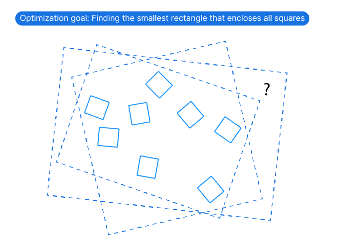
Let’s say we have a series of randomly rotated squares, and we want to find the smallest possible rectangle that contains all squares.
Here is the script setup: I drew the randomly rotated squares with a side length of about 0.5 in Rhino and referenced them to a Curve container. I also added a larger rectangle of 10 by 6 units around them – we’ll use this rectangle as the ‘canvas’ to limit the rectangle within.
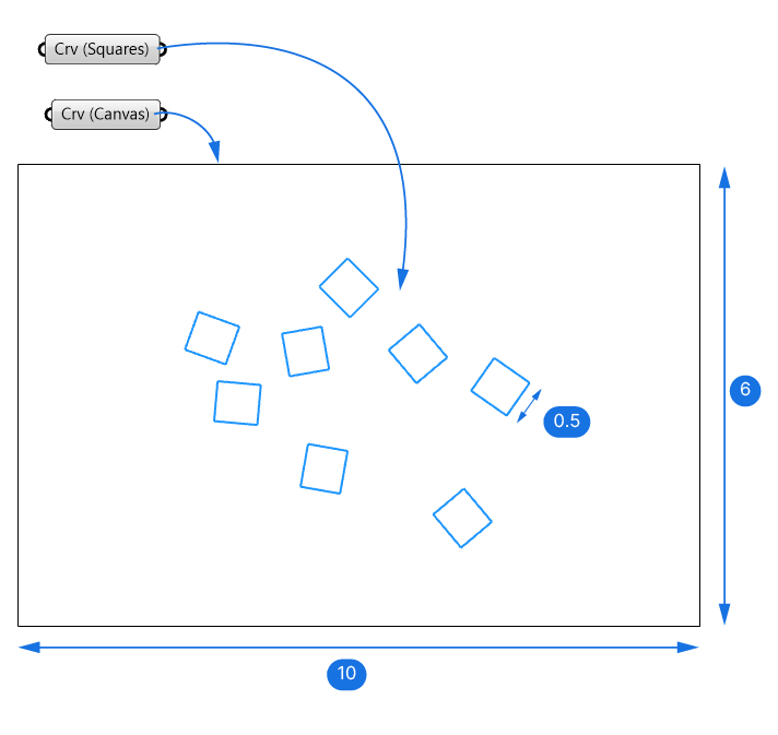
To use Galapagos to solve this problem, the first step is to create a parametric rectangle that we can control with Number Sliders. These Number Sliders will become the parameters (‘Genomes’) Galapagos will use to find the optimal solution.
Defining the Parameters
We want to create a parametric rectangle that can change the following parameters:
- the location (through x-and-y values)
- the width
- the height
- the rotation
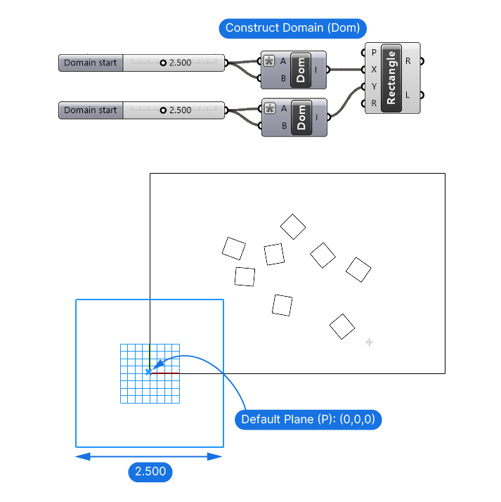
Let’s start by adding add a Rectangle component. It asks for a base plane, and the width and height in the form of domains (meaning a numerical range, for example -10 to 10).
Let’s start by defining the width and height. We’ll use a Construct Domain component to build a custom 2-dimensional domain, add a Number Slider with a range between 0 and 5 and a precision of three digits after the comma.
Connect the Number Slider to both the A and B input of the Construct Domain component, and then right-click on the A Input and enter the expression “-x” in the expression field. Doing so ensures the Number Slider will create a range from -x to +x, effectively centering the rectangle around the base plane.
Copy the Number Slider and Construct Domain component and connect it to the Y-input of the Rectangle.
These two Number Sliders now control the width and height of our rectangle.
Defining the BasePlane
Next, let’s define a parametric baseplane location.
To control the position of a point parametrically, we have to generate the point with x-and-y values. But creating a point using absolute x and y values is quite restrictive – if our model is far from the origin, the inputs become impossible to define and control.
That’s why we created our ‘canvas’ rectangle. We’ll turn it into a surface, and evaluate a point on that surface with reparametrized x – and y values. This means that we can describe any point on the surface with two values ranging from 0 to 1.
Let’s start by adding an Evaluate Surface component. Connect the curve (the component will turn the curve into a surface automatically because the curve is flat and closed), then right-click on the Surface ‘S’ input and select ‘Reparametrize’.
Next we’ll add two Number Sliders for the x – and -y values, and add a Construct Point (Pt) component, to connect the value to.
We can now use the resulting point as the uv-coordinate input of the Evaluate Surface component.
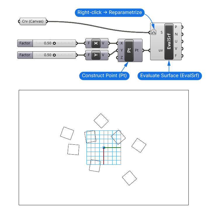
These two Number Sliders now allow us to parametrically describe any position on the surface (and thereby within the rectangle).
The evaluation parameters of 0.50 in the x -and y direction result in a point in the middle of our ‘canvas’.
Setting up the rectangle rotation
The last step is the rotation of the rectangle. The Plane (P) input of the Rectangle component defines both the location as well as the orientation of the rectangle. In other words the width and height will be defined in relation to the baseplane’s x and y axis.
So by rotating the baseplane, we can rotate the entire rectangle. Let’s go ahead and do that.
The Evaluate Surface component outputs the Frame ‘F’ at the evaluated point, which is a plane. Let’s connect this plane to the base plane input of the Rectangle.
Now let’s add a Rotate component (with the description ‘Rotate object in a plane’). The Geometry ‘G’ to rotate will be our Frame ‘F’. We want to rotate it on itself, so we can use the same Frame ‘F’ as the input for the Rotation Plane ‘P’.
Now let’s add another Number Slider to define the rotation of the plane in degrees. Set the Slider range to -180 to 180. Connect it to the Angle ‘A’ input of the Rotate component. Make sure to right-click on the Angle ‘A’ input and select ‘Degrees’ to tell the component that we are providing the rotation in degrees and not radians (the default).
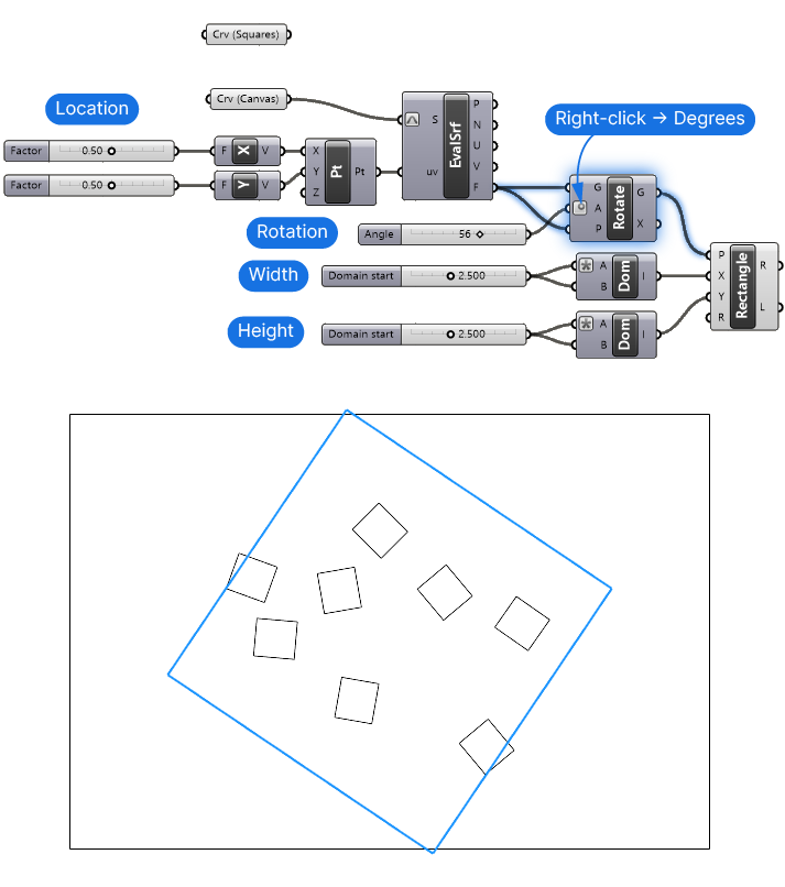
Our parametric rectangle is now ready! With the five Number Sliders we created, we can control the location, rotation and width and height of the rectangle!
Defining the Fitness
Now the interesting part begins – defining the fitness. Let’s think of how we can numerically express the optimal state we are trying to achieve.
We want the rectangle to enclose the squares as tightly as possible. In other words we want the smallest possible rectangle that still contains all squares.
Two parameters come to mind when it comes to evaluating the size of a rectangle:
- its area
- its circumference
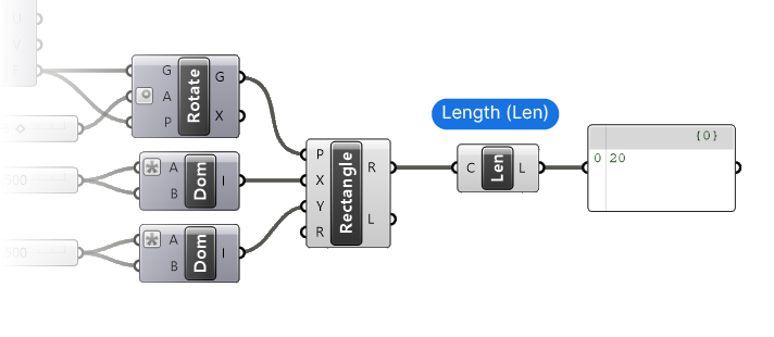
To keep it simple, let’s use the circumference. We can use the Length ‘Len’ component to get the length of the entire rectangle curve – that’ll do!
But we are not done yet:
Adding constraints – Penalizing unwanted solutions
If we just used this length as the fitness, Galapagos would optimize towards the smallest possible rectangle – without any additional constraints, the result would be a tiny rectangle with a length of 0!
We need to tell Galapagos that there is a second constraint: we want the rectangle to be small, yes, but it should also contain all the squares!
This is where penalization comes in. We are going to parametrically evaluate how many squares are outside the rectangle, and then multiple that number by an arbitrary larger number. Then we’ll add this number to the fitness value.
Since we will be optimizing for the smallest possible rectangle (and curve length) adding a high number will tell Galapagos that any solution containing squares are undesired or ‘bad genomes’ and it will optimize to avoid that. Not only that, since we are counting the number of squares that aren’t contained in the rectangle, the fewer it contains, the worse the fitness gets.
Let’s implement this penalization system!
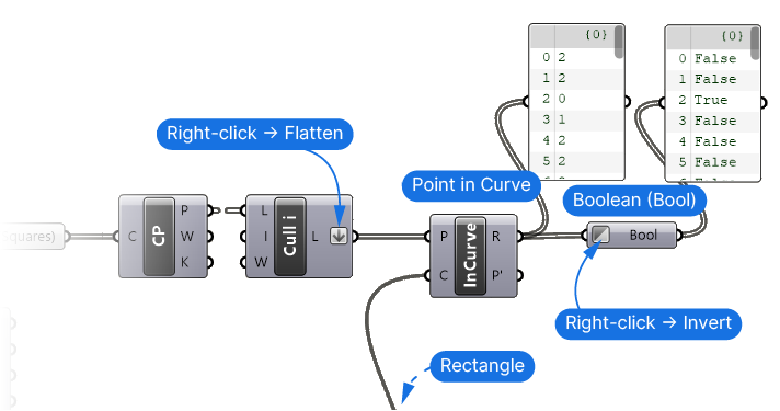
We already referenced our square curves – let’s start there. Since we want the rectangle to fully contain all squares, let’s evaluate the cornerpoints of the squares. Let’s add a Control Points (CP) component to extract them.
Keep in mind that a closed square has 5 control points, not just 4, the fifth just overlaps with the first to “close” the curve. Let’s remove that last point by using a Cull Index component and defining the index as -1. This leaves us with four points per square.
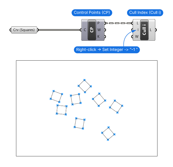
Let’s make sure to flatten the output of the Cull Index component, to get a single list with all the cornerpoints. Right-click on the output and select ‘Flatten’.
Counting the number of points outside the rectangle
Now let’s evaluate how many of those points are inside or outside the rectangle. To do that we’ll use the Point in Curve (InCurve) component. This component checks whether a point is within a closed curve.
Let’s connect the Rectangle component output to the Curve (C) input, and the Culled Points output to the Points (P) input.
The output is a series of numbers describing the Point to Region relationship.
- 0 = outside
- 1 = coincident
- 2 = inside
For us, it only matters whether it’s 0 or not. We can simplify this distinction by connecting the output to a Boolean (Bool) data container. It will convert any number that is 0 to ‘True’ and any other number to ‘False’. Let’s right-click on the component and toggle ‘Invert’. In doing so, we are now in a position to count the number of points that are outside the rectangle. That’s because ‘True’ and ‘False’ are just other words for 0 and 1.
By using the Mass Addition component we can sum up all numbers in the resulting list.
The Result (R) output of the Mass Addition component now contains the number of square corner points that are currently not contained in the rectangle.
To turn that number into a penalization, let’s add a Multiplication component and a Number Slider with a value of, say, 10,000. For the number to effectively deter Galapagos to consider it as desired solution, it should be significantly bigger than our normal fitness value, which is the rectangle curve length.
The last step is to add this multiplied number to the curve length.
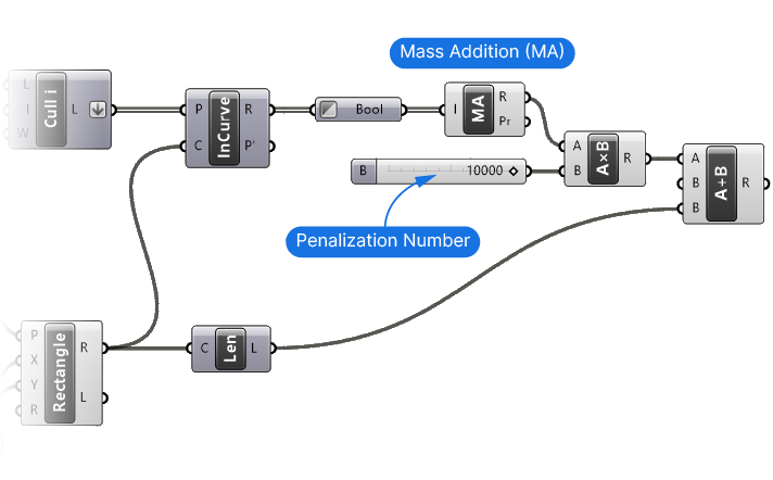
We now have a blended fitness number! A low fitness now accurately reflects our desired outcome.
Let’s now add Galapagos and run the solver!
Connecting Galapagos
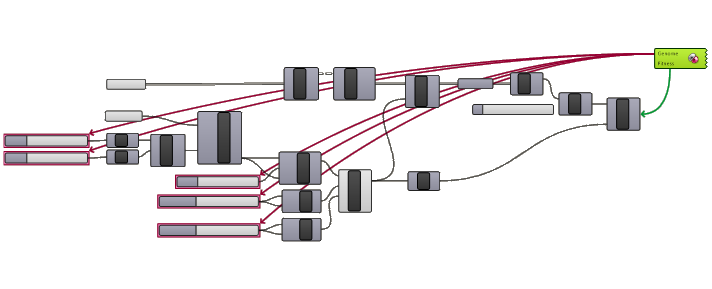
Now that everything is set up correctly, let’s add Galapagos to our Grasshopper script and connect the parameters and fitness.
Let’s connect the five Number Sliders controlling the rectangle to the parameters (‘Genome’) input. Remember to create the connection from the Galapagos component backwards, and make sure to hold ‘Shift’ to connect any additional Number Sliders.
Connect the fitness value the same way, dragging from the Galapagos component to the blended fitness value.
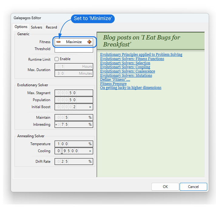
Running the Solver
Once everything is connected, double-click on the Galapagos component. The option tab opens. We want to optimize to the smallest value, so click the ‘minus’ sign to change the fitness target to ‘Minimize’.
Switch over to the ‘Solver’ tab. Pick the Simulated Annealing Algorithm (the Green ruby icon). I find that it works better for most optimizations. It generates more wildly different solution, while the Evolutionary Solver quickly narrows down the options, sometimes too soon.
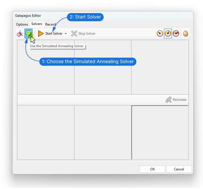
Click ‘Start Solver’ and enjoy the show!
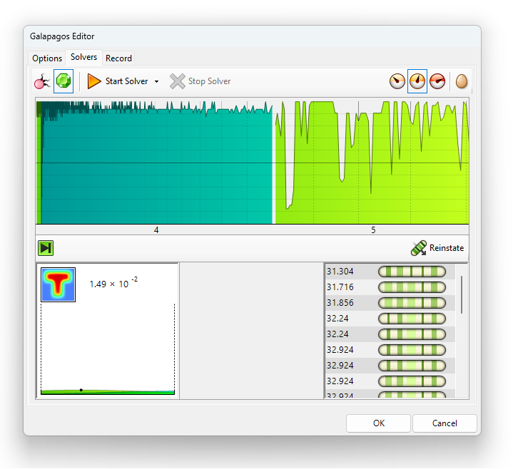
Galapagos will start iterating through options and you can lean back and watch it do the hard work! There is something incredibly satisfying in seeing it come closer and closer to the optimal solution.
The Simulated Annealing Algorithm will ‘restart’ over and over, trying different options, but don’t worry, once you hit ‘Stop Solver’, it will display the best option it has found up to that point.
When using this algorithm, avoid using the green genome window to reinstate other options. The best option is the one visible in the viewport. Click ‘OK’ to confirm. The Number Slider values will be adjusted to the ‘Genome’ or parameter constellation that led to the highest fitness.
After less than a minute, here is Galapagos’s result:
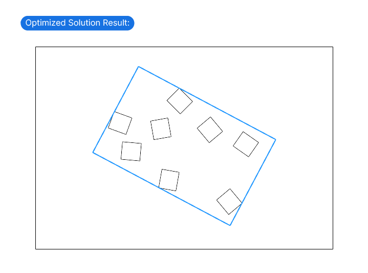
Pretty neat, right?
Tips & Troubleshooting – Things to Consider
Here are some things to consider when using Galapagos:
- Use Galapagos for solving complex problems where simpler methods don’t work. For example, finding the center of a triangle can be done quickly with basic geometry, which is faster and more accurate than using Galapagos. Save Galapagos for tasks that need you to adjust several parameters to get the best result.
- Narrow down the Ranges where possible: Galapagos works by generating a large number of variations. Calculating them all takes time. To avoid calculating unreasonable variations, narrow down the ranges of the Number Sliders to a range relevant for the task.
- Always manually check the Number Slider setup to ensure that the setup gives Galapagos all the degrees of freedom it requires to find the best solution. Sometimes a too narrowly chosen range can hinder the best solutions.
- Consider that the precision of the solution depends on the precision of the Number Sliders. If the Number Sliders have a precision of 1.0, you’ll get a rougher result than if it is 1.000. But again, this will increase computation time.
- For complex, multi-parameter problems, consider enabling the runtime limit in the options tab; this setting ensures the process stops automatically after a specified amount of time.
- Always double-check the result – is it really the optimal solution or is the fitness not setup correctly?
Concluding thoughts on Galapagos in Grasshopper
Galapagos significantly extends what we can do in Grasshopper, almost deserving to be a plugin on its own. This powerful little tool can help you solve complex problems efficiently.
A last word of advise: Don’t overuse it! While it’s satisfying to watch it work for you, try to find a deterministic solution to your problem first. More often than not it’s a better way to go about it!
Happy designing!